3. Notebooks with Python – part 2

In this post, we will create a third notebook to prep and transform the wta_matches csv’s.

Matches Notebook

Launch the Databricks portal and create a new cluster, as shown in the previous post. Name the cluster matchesNotebook.

Recall from the previous posts on ADF, that we have ingested the wta_matches files (53 in total) in the landing/matches folder of our data lake.

1. Accesing ADLS gen2 storage from Databricks

We have seen previously that we need to set the data lake context at the start of the notebook session. Let’s start by writing the code to access the data lake storage using the key1 storage account access key. Check the previous post to recall how to locate the key1 access key.

#access Azure Data Lake gen2 directly using storage account key
accountName = "dlswta"
#copy your key1 account key between the double quotes
accountKey = "<copy-paste-your-key1>"
config = "fs.azure.account.key." + accountName + ".dfs.core.windows.net"

spark.conf.set(config, accountKey)

You need to run this code at the beginning of the session, or each time you restart the cluster. Press the Run button to Run Cell or use the Shift+Enter shortcut.

2. Read data

Explore the content of the landing/matches folder using the dbutils.fs.ls command.

dbutils.fs.ls("abfss://landing@dlswta.dfs.core.windows.net/matches")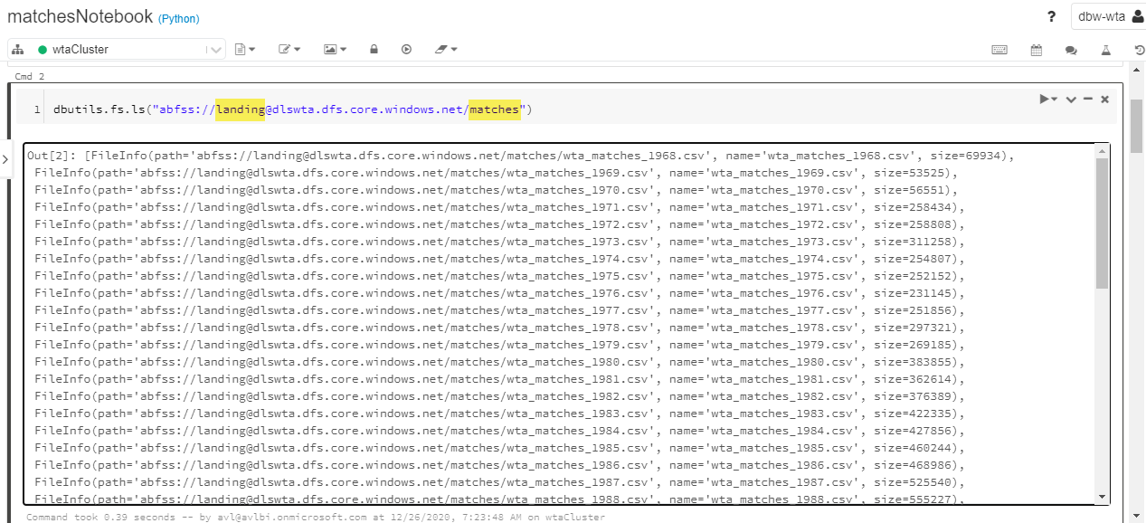

Load the files into a dataframe using either *.csv or wta_matches_*.csv in the file path. The wta_matches files contain header on first row. Set the header option to True and inferSchema option to True, to let Spark automatically determine the column data types.

#set the data lake file location
#filePath = "abfss://landing@dlswta.dfs.core.windows.net/matches/*.csv"
filePath = "abfss://landing@dlswta.dfs.core.windows.net/matches/wta_matches_*.csv"

#read the data into df dataframe
df = spark.read.csv(filePath, header=True, inferSchema=True)
display(df)

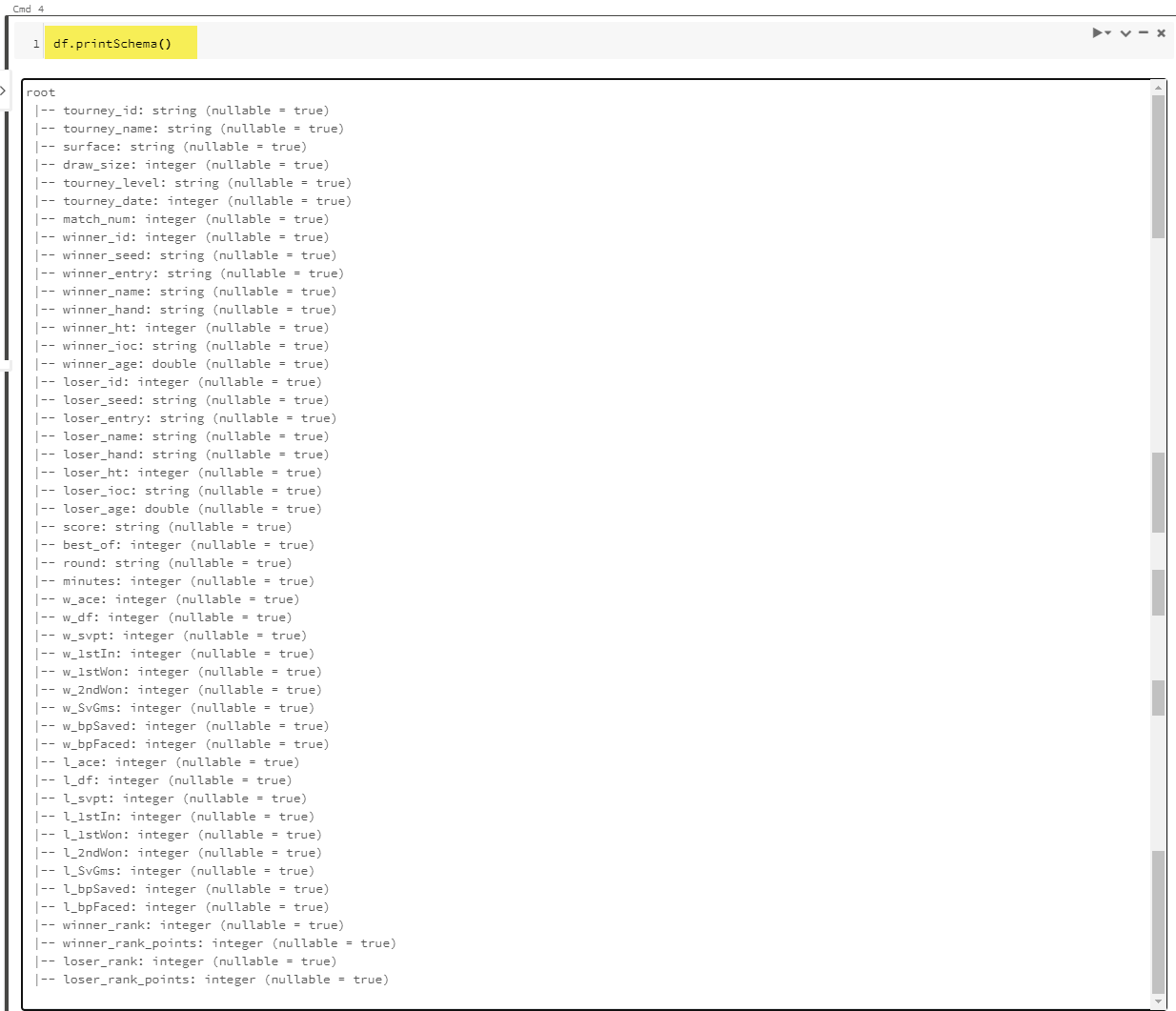
Use the printSchema() command to see the inferred data types.

Issue the count() command to get the total number of rows. There are 125580 entries in all wta_matches files.

3. Perform SQL queries on Spark dataframe

Instead of using PySpark to operate on the dataframe we can write SQL queries. One option is to create a temporary view on top of the dataframe. Issue the createOrReplaceTempView command and pass the name of the view as parameter.

#creating a temporary view that we can query using SQL
df.createOrReplaceTempView("vw_matches")

Use the %sql magic command and start writing some quick SQL queries to view and operate on the data..

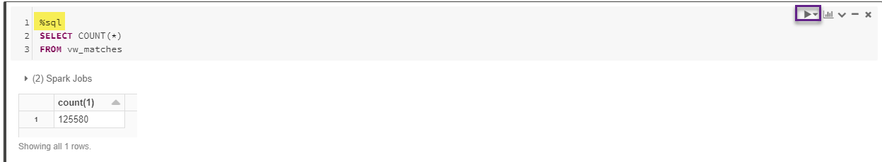
Let’s write a query to count the number of rows.

%sql
SELECT COUNT(*)
FROM vw_matches

Run Cell returns 125580.

Explore the data by writing more complex SQL queries. For example, you can use the query below to see a subset of the data using some filters.

%sql
SELECT tourney_name
  ,tourney_date
  ,match_num
  ,winner_name
  ,winner_ioc
  ,loser_name
  ,loser_ioc
  ,score
FROM vw_matches
WHERE winner_name='Bianca Andreescu'
ORDER BY tourney_date DESC, match_num DESC

Run Cell and explore the result.

4. Write processed data

Issue the df.coalesce(1).write.csv() command to save the data to the cleansed zone of our data lake.

destPath = "abfss://cleansed@dlswta.dfs.core.windows.net/matches"

#write the data to the new location forcing one partition
df.coalesce(1).write.csv(destPath, header="true", mode="overwrite")

Back to Azure Portal, navigate to your data lake Storage Explorer to explore the new data in your data lake. Note the auto generated files for process tracking and the actual csv file containing the data.

The matchesNotebook we created in this post is available on github here.

What’s next
Next stop in our journey is Power BI. We will use the files we just saved in the cleased area of the data lake to create a data model in Power BI. Follow the Power BI series to write reports and get insights about WTA matches and players.🐳

Want to read more?
Microsoft learning resources and documentation:
Apache Spark Tutorial: Getting Started with Apache Spark on Databricks

---