Let’s create a WTA Grand Slam data model for Power BI!

For this post I want to create a tabular data model in Power BI containing WTA Grand Slam tennis data.

To give you a flavor of what we want to achieve, the visual diagram below shows the data model.

But to get the data in this format, we have to do some work. A typical workflow is shown below.

In Power BI Desktop, we will connect to the data source, use Power Query to shape and transform data, create relationships to connect the tables in the model and use DAX to enhance the data model.

Know your data – A bit of tennis history

There are 4 Grand Slams that take place every calendar year: Australian Open, French Open (Roland Garros), Wimbledon and US Open.

The Australian Open was first known as the Australasian Championships. It became the Australian Championships in 1927. Then, in 1969, it became the Australian Open. The tournament is the first of the four Grand Slam tennis events held each year, preceding the French Open, Wimbledon, and the US Open.
The Australian Open is held in Melbourne, Australia. It starts in the middle of January and continues for two weeks.

The French Open, also known as Roland-Garros, was founded in 1891 and referred to as the French Championships. It is chronologically the second of the four annual Grand Slam tournaments, occurring after the Australian Open and before Wimbledon and the US Open.
The French Open is held at the Stade Roland Garros in Paris, France. It starts in late May each year and continues for two weeks.

The Wimbledon Championships, commonly known simply as Wimbledon, is the oldest tennis tournament in the world, founded in 1877, and is widely regarded as the most prestigious. Wimbledon is the only major still played on grass, the traditional tennis playing surface.
The Wimbledon Championships is held at the All England Club in Wimbledon, London. It takes place over two weeks in late June and early July.

The US Open is a hardcourt tennis tournament founded in 1987. It has been chronologically the fourth and final grand slam tournament of the year. 
The US Open is held in Queens, New York. It starts on the last Monday of August and continues for two weeks.

The data source

I’m gonna use as data source the tennis_wta csv files available on Jeff Sackman‘s github. Jeff Sackman has done a wonderful job, scraping the WTA’s website and collecting the available data resources into an extensive database of match results. His work is licensed under a Creative Commons Attribution-NonCommercial-ShareAlike 4.0 International License.

Download the following csv files and store them in a folder on your local drive.

• match result files – containing all tour-level single matches of a season and have the filename format wta_matches_yyyy.csv
• players file – one file, named wta_players.csv
• ranking files – all ranking files

M like in MashUp

Head over to Power BI Desktop and from the Home ribbon bar, choose Transform data to open Power Query. We use Power Query to shape the data into the format and structure we need. Common data shaping tasks are: rename/remove tables and columns, remove rows, changing data types, merge/append queries, pivoting/unpivoting, splitting column by delimiter, etc.

Many of the transformations in Power Query editor can be done using options in the ribbon bar. More complex transformations will require to manually edit some code in Power Query M Formula Language.

M is a functional, case-sensitive language, optimized for writing data mashup queries.

First, I’ll define a parameter for the folder path where I’ve downloaded the tennis_wta csv files.

Once you hit OK, the newly created parameter will appear in the Queries panel. Let’s connect to the source folder, by clicking New Source in the Home ribbon bar and then select Folder in the Get Data window.

In the Folder path, select the parameter you’ve created above.

In the SourceFolder window, hit Transform Data.

The new query that is created contains all files in the source folder. I filtered the query to only keep the csv files and named it Tennis WTA Data Source. I also disabled the Enable Load option. This is going to be the base for all other queries.

Next, I’ll create a reference to the Tennis WTA Data Source and use it to create the Player query.

• In the Query Settings window, name the query Player
• Filter the column Name, and select the wta_players.csv file (we have only one player csv file!)
• The Content column, of type Binary, contains the content of the wta_player.csv file. I’m gonna add a custom column and use the Csv.Document() function, to get the data from the csv file.
  I’ll pass as argument the Content column. Basically, we’re saying: interpret the Content as csv format and return a table of rows and columns of data.
  For more information on the Csv.Document() function check the Resources section below.
• Keep only the Custom column created above and remove all other columns.
• At this point, you could expand the Custom column by clicking the arrows icon on the column header. I prefer instead to use the Table.Combine() function. As the name suggest, this M function will combine several tables. Obviously, for the Player query, we have only one table. The use of this function will become more clear when loading the match csv files. For now, let’s keep the code consistent with the other queries we’ll write.
• Promote the headers and spend some time to understand the data. Then, change the data type for the columns below:

column name	data type
player_id dob height	Whole number Date Whole number

• Note that changing the data type to Date for the dob column, resulted in some errors. This is because we had a value (19000000) that could not be converted to a valid date. Replace the error with null.
• Merge the name_first and name_last columns in one single column: Player Name.
• The last thing I’m gonna do is to rename the columns and give them more user friendly names.

From the Home ribbon bar, choose Advance Editor and observe the M query that was generated for each of the steps above.

You can watch all the steps applied in the video below.

Let’s create another reference to the Tennis WTA Data Source and use it to create the Ranking query.

• Once the reference query created, name it Ranking.
• This time I’ll filter based on a condition, and we want to keep all rows where the Name column begins with “wta_rankings”. Per the time I write this blog post, there are six ranking csv files. The files contain player WTA rankings over time.
• Add a custom column and use the Csv.Document() function, to get the data from the csv file.
• Keep only the custom column created above. Remove all other columns.
  We have only 6 rows, of type Table, one for each of the ranking files we loaded.
• Use the Table.Combine() function to combine all 6 tables.
• Use the first line as header.
• Keep the columns below and change their data type as follows:

column name	data type
ranking_date rank player points	Date Whole number Whole number Whole number

• When profiling the data based on the entire dataset, we see there are errors on the ranking_date column because some of the data could not be converted to the Date type. Remove all rows with errors.
• Lastly, rename the columns and give them more user friendly names.

Here’s the M code generated for the steps above.

You can watch all the steps applied in the video below.

Starting again with the Tennis WTA Data Source, I will now filter only the wta_matches files. I want to create another base query, containing only the grand slam matches. I will then reference it and create a Matches query and a Tournament query.

Let’s create the Grand Slam Matches query first.

• Once the reference query created, name it Grand Slam Matches.
• Filter to keep all rows where the Name column begins with “wta_matches” and does not contain “qual” (we don’t include the qualification matches).
  At the time of writing this post, there are 103 remaining wta_matches files.
  The files contain information about the WTA tournaments and matches over time.
• Add a custom column and use the Csv.Document() function, to get the data from the csv file.
• Keep only the custom column created above. Remove all other columns.
• Use the Table.Combine() function to combine all 103 tables.
• Use the first line as header.
• Filter the tourney_level column for value “G”. This will filter the dataset and keep only the grand slam matches.
  There are 4 Gand Slams that take place every calendar year: Australian Open,
  French Open (Roland Garros), Wimbledon, US Open.
• I also did a quick data profiling on column tourney_name and noticed that we need to correct some values.
  I’ve replaced “Australian Open 2” with “Australian Open” and “Us Open” with “US Open”.
• Control+click to select the following columns and choose Remove
  “winner_seed”, “winner_entry”, “winner_name”, “winner_hand”, “winner_ht”, “winner_ioc”, “winner_age”, “loser_seed”, “loser_entry”, “loser_name”, “loser_hand”, “loser_ht”, “loser_ioc”, “loser_age”, “best_of”, “w_ace”, “w_df”, “w_svpt”, “w_1stIn”, “w_1stWon”, “w_2ndWon”, “w_SvGms”, “w_bpSaved”, “w_bpFaced”, “l_ace”, “l_df”, “l_svpt”, “l_1stIn”, “l_1stWon”, “l_2ndWon”, “l_SvGms”, “l_bpSaved”, “l_bpFaced”, “tourney_level”, “draw_size”
• Right click the query name and uncheck Enable Load.

Here’s the M code generated for the steps above.

You can watch all the steps applied in the video below.

Next, I’ll create the Tournament query.

• Create a reference of the Grand Slam Matches query and name it Tournament.
• Keep the following columns: tourney_id, tourney_name and surface. Remove all other columns.
• Use the functionality Transform>Extract>Text Before Delimiter to extract the tournament year from the tourney_id column.
  The year value is the first part of the string value, before the “-“.
  Rename the column tourney_year.
• At this point we have many duplicates. There’s a row for each match in a tournament, for every year. Let’s remove duplicates.
• We now have one row for each pair (tournament, year, surface).
  Let’s take as example the Australian Open. It was played on Grass surface until 1987 and on Hard surface since 1988.

Based on this information, I want to keep only two rows for Australian Open:
– one row for surface type Grass: Australian Open, Grass, 1969
– and another for surface type Hard: Australian Open, Hard, 1988
For the tourney_year, I’ll keep the year when the tournament was first played on that specific type of surface.

To achieve this, I’ll use the Group By functionality in Power Query.

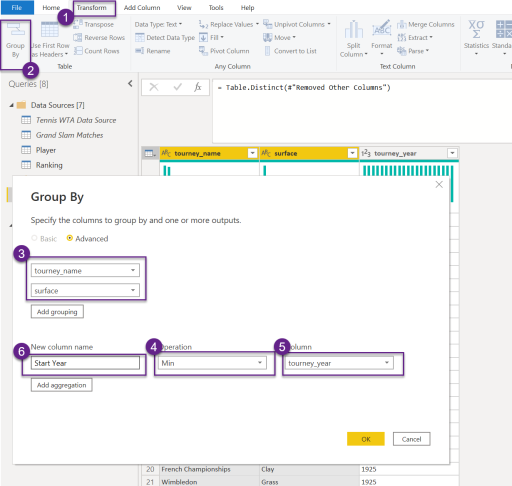
This will result in distinct pairs of (tourney_name, surface, Start Year)

• Let’s add an index column using the ribbon bar options Add Column>Index Column>From 1 and name it Tournament Id
• Change the data type and rename the columns to more user friendly names.

Here’s the M code generated for the steps above.

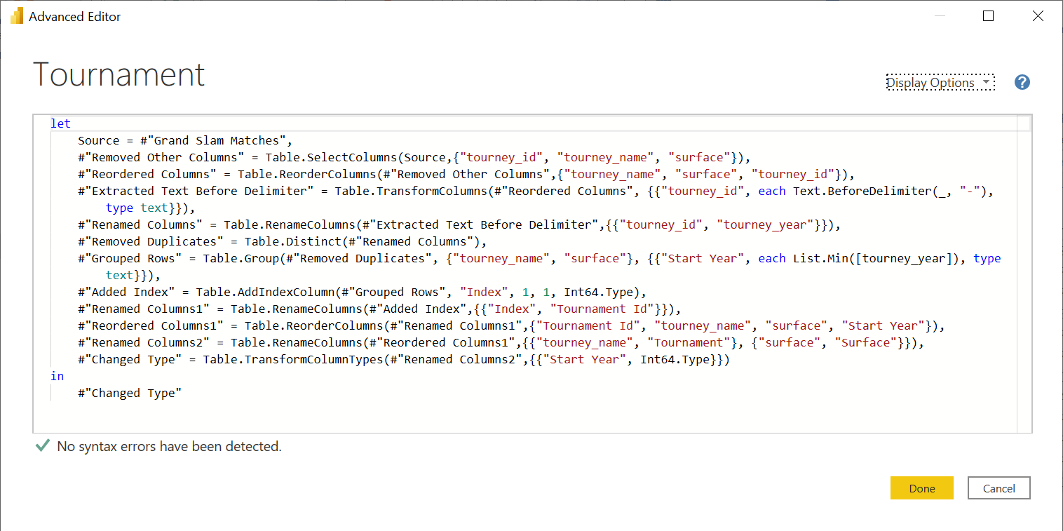
You can watch all the steps applied in the video below.

Lastly, I’ll create the Matches table.

• Create a reference of the Grand Slam Matches query and name it Matches.
• This table will have one entry for each match of any tournament. I’ll start by creating a reference to the Tournament Id in the Tournament table (query) created above.
  To achieve this, we’ll use the Merge Queries functionality in Power Query. The matching columns are tourney_name, surface and Tournament, Surface respectively.

• Expand the merged query and keep only the Tournament Id column

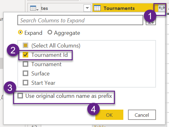
• Now we can remove “tourney_id”, “tourney_name”, “surface” columns, since we this information in the Tournament table and we just brought in the reference column Tournament Id
• All is left is to change the data type and rename the columns.

New column name	Old column name	Data type
Tournament Id Tournament Date Match No Winner Id Opponent Id Score Round Minutes	Tournament Id tourney_date match_num winner_id loser_id score round minutes	Whole number Date Whole number Whole number Whole number Text Text Whole number

Here’s the M code generated for the steps above.

You can watch all the steps applied in the video below.

We have created all tables in Power Query; we are now ready to Close&Apply and return to Power BI Desktop.

Data modeling & DAX

Back in Power BI Desktop, head over to the Data view and explore the four tables we’ve just created in Power Query.

Make it a habit to add a Date table to your model even when it is not immediately obvious that you need one. In most of the cases (if not always) your model needs a Date table (dimension)!

I’ll use DAX to add a Date table. In the Data view, go to Table tools and click New table, then add the following DAX statement.

• Make sure the Date type of the Date column is set to Date and the Format is mm/dd/yyyy

• Make sure the Data type of the yyyymm and MonthNum columns is set to Whole number.
• Set the MonthName and Month columns to Sort by column MonthNum.
• Set the Year Month column to Sort by column yyyymm.

• Lastly, right click the Date table and choose Mark as date table.

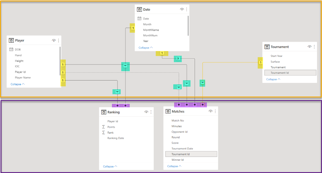
We are now ready to go to the Model view and add relationships to our model. Add the following relationships to the model:

Dimension	Fact	Relationship type
Date [Date]	Matches [Tournament Date]	1 – * (One to many)
Player [Player Id]	Matches [Winner Id]	1 – * (One to many)
Player [Player Id]	Matches [Opponent Id]	1 – * (One to many) Inactive relationship
Tournament [Tournament Id]	Matches [Tournament Id]	1 – * (One to many)
Date [Date]	Ranking [Ranking Date]	1 – * (One to many)
Player [Player Id]	Ranking [Player Id]	1 – * (One to many)

Here is the data model diagram.

Now, let’s add a Measure table to our model. A measure table is a disconnected table (has no relationship with other tables) and is used to group in one place all the DAX measures.

On the Home ribbon bar, choose Enter data and give your table a name (Measures table or DAX for example), then add a measure. Instead of creating a dummy measure, I’ll create two measures to return the Winner Name and the Opponent Name.

Recall that the Player table has two relationships with the Matches table, of which only one can be active at a time. We’ve created an active relationship Player[Player Id] – Matches[Winner Id], and an inactive relationship Player[Player Id] -Matches[Opponent Id].

Delete the Column1 that was automatically added when you created the table. Keep only the measures we’ve just created. The DAX measure table has now a new calculator icon, and it will always be listed at the top in the Fields pane.

Save and name the pbix file WTA Grand Slam Model. The model is now ready to be published to Power BI Service.

We can then create a new pbix file for report visualizations and connect it to the published WTA Grand Slam Model.

You can download the model from my github.

Resources

• Chris Webb’s BI Blog : An In-Depth Look At The Csv.Document M Function

*This post was revised and updated on October 14, 2022

---